It’s been a year since the last post now. My drafts pile is growing taller by the week. Let’s see if this one gets published.

Bayesian Incompleteness?
Just like last time, I’m here to try my unprofessional and woefully unread hand at a topic that has likely been explored in depth by academics. Hoping my feeble attempt at self-awareness serves as a facade for this manifestation of Dunning-Kruger, let me introduce and name a concept that very likely already has one: the Bayesian Incompleteness Condition (or Fallacy). The pretension and audacity ostensibly baked into that name undermines how common of an experience it is. A BIC refers to a situation in which a subject draws an incorrect conclusion about a particular population because of the lack of a crucial conditional in one’s consideration. The subject uses an empirical assertion about a broader group which that population is a member of. However, including the crucial descriptive conditional would reveal that the broader observation does not apply to the population subset in question.
I use the term “Bayesian” here because it’s based on, and perhaps most evident using, examples of Bayesian probabilities. Let’s make this concrete with an example. Say we discover the median individual income in Canada is $65,000. Then, we visit a small, homogenous, mining town in northern Ontario and are shocked when a comprehensive survey reveals a much lower local median income. Does this mean we made a systematic error in setting up our survey? You can probably see why the answer is “no”. Even though the nationwide median income is $65,000, the nation is composed of countless subgroups with their own unique characteristics. In fact, one should expect that isolating a very specific subgroup within a larger population will reveal at least some characteristics that are not reflected in the average member of the wider population.
There are countless absurd examples of Bayesian Incompleteness Conditions that one can come up with, but the fact that a BIC can also be subtle means they are not to be dismissed. You might visit the Sonoran Desert and expecting a temperature of fourteen degrees Celsius because that’s the average surface temperature of the Earth. You might visit Silicon Valley and think everyone is embellishing their resumes because the average American doesn’t have such qualifications. Although these are valid examples in their invalidity, BICs can be far more reasonable sounding. To “steelman” the BIC position for a second: maybe we can accept that there are deviations from the average within a population, but sometimes, the results we observe are so far outside our expectations for the wider group (perhaps several standard deviations, to use a variability metric), that the limits of Central Limit Theorem are seriously tested. Sure, maybe we can accept that the average income in the small mining town will differ from that of Canada as a whole, but if its variability is beyond a certain threshold of standard deviations – whether that be two, three, or more – from what we observe nationwide, then maybe there’s a problem to be resolved. The most succinct answer to this concern lies in looking at this problem through the lens of sampling error.
The Sampling Error Lens
In statistics, there exists the concept of an underlying population you are investigating. This population is usually immeasurable in its entirety, so we instead draw samples from it and use them to make inferences about the underlying population. Intuitively, the samples we draw should probably be subject to constraints, ensuring they do a good job of representing the population we’re trying to study. The theoretical idea is that using a sample that is not representative actually provides information about a different abstract “population” than the one you care about.
Recognizing this, if we return to the northern Ontario mining town example, we can see more clearly what we are doing wrong. By assuming the data we collect from the town should line up with nationwide statistics, we are buying into the implicit premise that the mining town should be a representative sample for Canada as a whole. We know this cannot be the case; there are almost certainly a range of characteristics that the people in the mining town share that are vastly over- or under-represented compared to the national population. These can be super obvious. For example, the mining town probably contains a much higher proportion of miners compared to the total Canadian population. There is also the straightforward problem of representation of people from Ontario (or northern Ontario, or even this specific town, etc.) compared to the national population. The point is that the key differences between the characteristics of the mining town and the total Canadian population means that the mining town is simply not a representative sample of the population we’re interested in.
Now this might be hard to wrap your head around so don’t worry if you don’t get it because it’s not super necessary: using the mining town’s statistics to draw conclusions would actually be an exercise in describing a completely different population, one that is non-existent and appropriately represented by the sample.
The Bayesian Lens
Let’s introduce the Bayesian model to reframe this problem. The Bayesian perspective is an attitude that views probability as the chance of a particular event occurring given the knowledge of certain “priors”. It is not possible to know and account for every single prior in a situation, but the more priors that are included in one’s calculation, the more accurate the final probability is to the specific situation at hand. Here’s an example: imagine you are pulling marbles out of a bag. At the start, you are aware that there are five red marbles and five black marbles inside the bag, so you arrive at the correct conclusion that there is a 50% chance you draw a black marble. However, after drawing the first marble, this probability no longer reflects reality because the very population you are drawing from (the marbles inside the bag) has fundamentally changed. If you drew a black marble first, there is a greater likelihood you will draw red the second time. Although we started with 50-50 odds, we are now aware of a crucial “prior” that we must account for, which is the fact that one black marble has already been drawn from the bag.
In a Bayesian framing, we could model this scenario as a probability with an encrypted conditional that accounts for the prior. In mathematical terms, the original probability could be written as such:
P(B) = 5/10 = 1/2
The above simply states that the probability (P) of drawing a black marble (event B) from the bag is 1/2. To add in the prior as a conditional:
P(B|-1B) = 4/9
The “|” symbol is used to denote a conditional event, which I’ve labelled as “-1B” in this case to indicate one black marble having been drawn already. The resulting probability is 4/9 – less than 5/10 because of the now-disproportionate distribution of black and red marbles inside the bag.
This example is just meant to demonstrate the broad concept of Bayesian probability and show that accounting for crucial priors can alter an evaluation of an event’s likelihood. The way I’m applying this idea to statistics is very similar. We can use broad statistics about large populations, but only insofar as forming a generalized view of that population as a whole. Dealing with a specific subset of that population is a totally different case because there are key priors at play that can affect those statistics. Ignoring these priors leads to naive and incorrect conclusions. Assuming the average Mexican man weighs sixty-five kilograms because that’s the average mass of a human ignores key prior characteristics of being a Mexican and a man. Assuming you can go out in a t-shirt if you live in Vladivostok, Russia just because the average world temperature is fourteen degrees Celsius ignores the key prior of being located in Vladivostok. And assuming the average adult in the northern Ontario mining town earns $65,000 a year ignores a number of key priors, all ultimately amounting to being located in a very specific part of the country with disproportionate characteristics.
At the same time, paying attention to as many priors as possible should yield the most accurate statistics. If you have a male Arab software engineer living in Vancouver, using the raw national income numbers to draw conclusions about him would be naive. But we can narrow down our scope one characteristic at a time. What about the average income for males across Canada? A little better. What about the average income for male Arabs across Canada? Better still? Add in the priors of living in Vancouver and being a software engineer and you’d eventually get a pretty compelling number to use as an estimate for the man in question.
Data Collection vs Data Use
This is where I tie the two angles together; the sampling error framework and the Bayesian framework are two sides of the same coin, merely two different mental approaches to the same problem. Through one lens, the misuse of national census statistics in a specific mining town is an issue because the mining town is not representative of the national population. Through the other lens, it is because national census data does not account for the key prior knowledge we have of the specific population subset we’re investigating. If you now collected data on a narrow population subset, such as northern Ontario miners, it would be a different story. Your sample would now be representative of the population (sampling error perspective) and you would have accounted for multiple key priors (Bayesian perspective).
At this stage, the question that remains is: why is the Bayesian perspective useful? The reason lies in the nature of how we use statistics compared to how we collect statistics. Collecting statistics on any particular “broad population” requires sampling. In this process, it is the population we’re actually interested in and the sample we use is just a tool to learn more about it. However, when we are using statistics to come to some kind of conclusion, we are working backwards. Someone has already collected statistics about a broad population from (hopefully) representative samples and we use them to draw conclusions about narrow, representative subsets of the population.
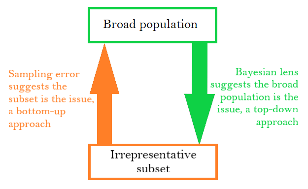
In a case like that of the mining town, where there is a mismatch between the population and the subset, we can choose to focus on either the subset being too irrepresentative – the sampling error perspective – or the population being too broad – the Bayesian lens. The former perspective implies we are using the wrong subset and if we changed it to make it more representative, we could resolve our issue. This makes sense if we are collecting data about the underlying population because we have a fixed population in mind that we want to investigate. Changing the population itself would not make sense if we have such a specific goal in mind. However, for data application, this is a counter-productive perspective. Because it is the population subset that we wish to learn more about, it would make little sense to emphasize the way in which the sample does not represent the population. In the mining town example, it is unhelpful to emphasize the fact that the town does not represent Canada as a whole because it does not point to how we can go about solving the issue at hand. What we can do instead is to point out that the statistic we are using is from too broad of a population. This explains more succinctly what the issue and it is now apparent that we can solve the problem by using statistics from a much narrower population.

All of this long-winded discussion is to say this ultimately: the Bayesian Incompleteness Fallacy is both: a) a common misuse of statistics that should be avoided; and b) a useful perspective to apply when trying to use statistics to draw conclusions. The sampling error lens is also useful, but I think it makes much more sense to apply when performing data collection and your population of interest is fixed. So, look out and be cautious enough to ensure that you’re accounting for sufficient key priors when using statistics.
The average person is alright. But if you made it this far, I’m going to update my priors and confidently say that you are a true legend. As always, come back for the next one in twelve months.
